Definição do problema

library(cmpreg)

## Loading required package: bbmle

## Loading required package: stats4

data(nematodes)
str(nematodes)

## 'data.frame':    94 obs. of  5 variables:
##  $ cult: Factor w/ 19 levels "A","B","C","D",..: 1 1 1 1 1 2 2 2 2 2 ...
##  $ mfr : num  10.52 11.03 6.42 8.16 4.48 ...
##  $ vol : int  40 40 40 40 40 40 40 40 40 40 ...
##  $ nema: int  4 5 3 4 3 2 2 2 2 2 ...
##  $ off : num  0.263 0.276 0.161 0.204 0.112 ...

## help(nematodes, h = "html")

##======================================================================
## Análise de dados de nematóides
xyplot(nema ~ off, groups = cult,
       type = c("g", "p"),
       data = nematodes,
       auto.key = list(
           title = "Linhagens",
           cex.title = 1,
           corner = c(0.9, 0.9)
       ))

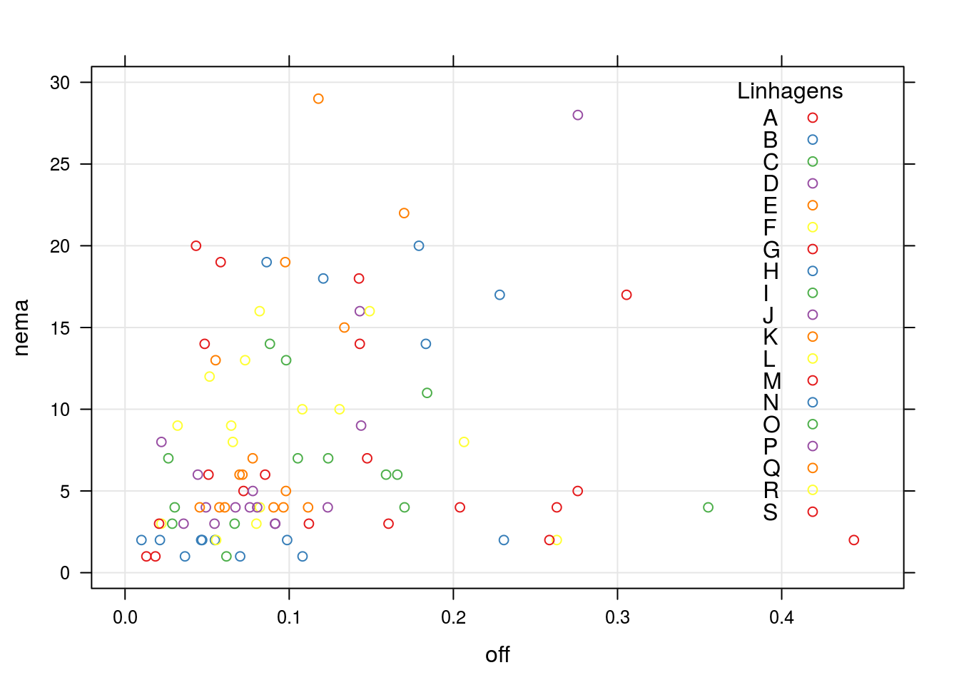
Duas estruturas para modelagem serão consideradas * Modelar somente o efeito aleatório das linhagens, * Modelar somente o efeito fixo de off e aleatório das linhagens.

Modelos em competição

Modelo misto Poisson (ajustado pela maximização da verossimilhança)
Modelo misto COM-Poisson (ajustado pela maximização da verossimilhança)
Modelo misto Poisson (sob o paradigma Bayesiano)
- INLA (Integrated Nested Laplace Aproximation)
- Amostragem MCMC (usando o jags)
Modelo misto Gamma-Count (sob o paradigma Bayesiano - INLA)

Abordagem de Máxima Verossimilhança

Modelo misto Poisson

##----------------------------------------------------------------------
## Com a Poisson
library(lme4)

## Loading required package: Matrix

mle0 <- glmer(nema ~ (1|cult), data = nematodes,
              family = poisson)
mle1 <- glmer(nema ~ log(off) + (1|cult), data = nematodes,
              family = poisson)

##-------------------------------------------
## Estimativas dos parametros
## Para o modelo sem efeito fixo
tmle0 <- rbind(sigma = c(sqrt(VarCorr(mle0)$cult), NA, NA),
               summary(mle0)$coef[, -4])
rownames(tmle0)[2] <- c("(Intercept)")
tmle0

##             Estimate Std. Error  z value
## sigma       0.759144         NA       NA
## (Intercept) 1.760503  0.1808152 9.736474

## Para o modelo com efeito fixo
tmle1 <- rbind(sigma = c(sqrt(VarCorr(mle1)$cult), NA, NA),
               summary(mle1)$coef[, -4])
tmle1

##              Estimate Std. Error  z value
## sigma       0.7310786         NA       NA
## (Intercept) 2.1562623 0.23278215 9.263005
## log(off)    0.1620083 0.06397819 2.532242

## Predição dos efeitos aleatórios
ranef.mle0 <- data.frame(ef = ranef(mle0)$cult[, 1], m = "mle0")
ranef.mle1 <- data.frame(ef = ranef(mle1)$cult[, 1], m = "mle1")
ranef.mle <- rbind(ranef.mle0, ranef.mle1)

densityplot(~ef, groups = m,
            data = ranef.mle,
            axis = axis.grid,
            auto.key = TRUE)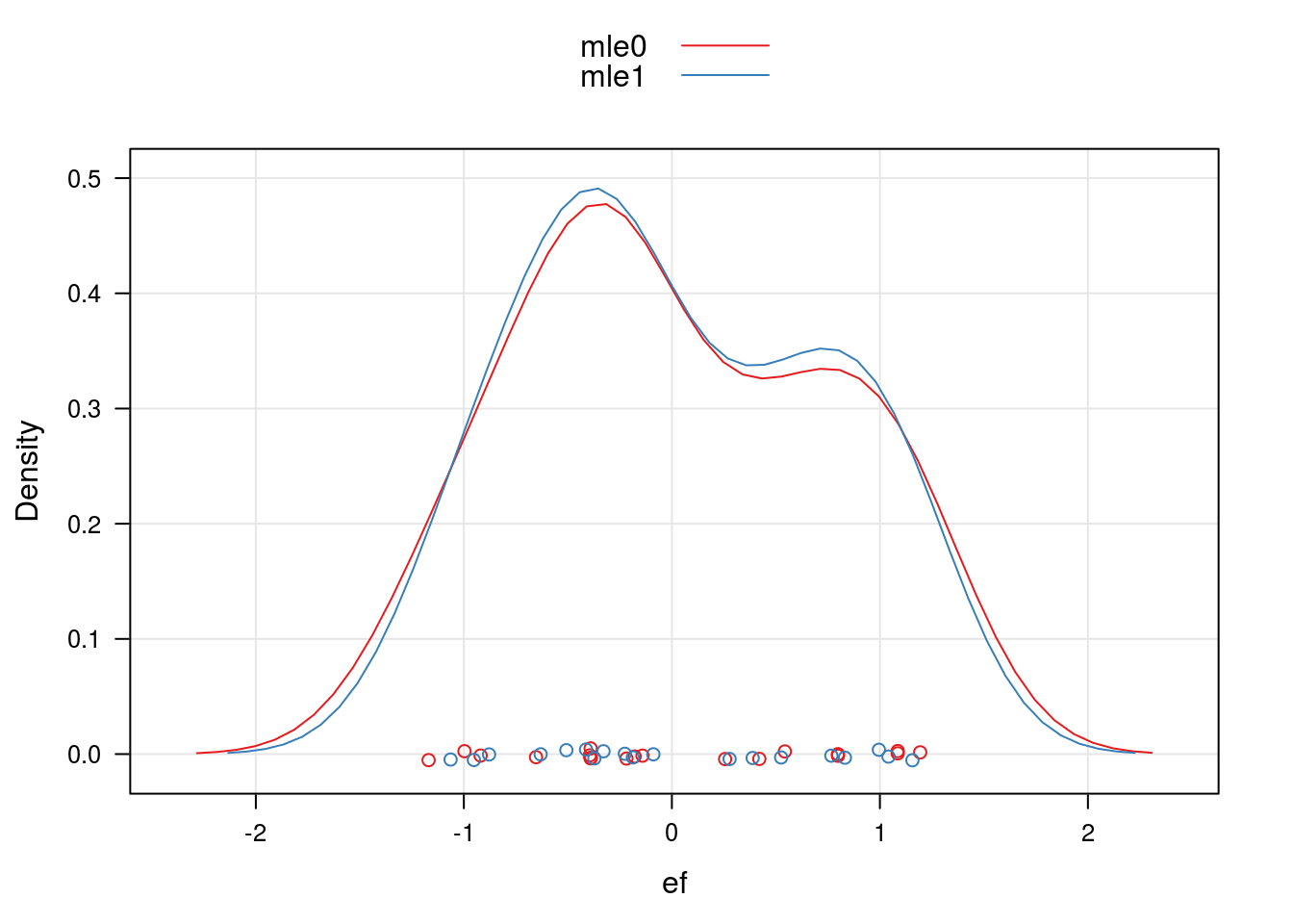

Modelo misto COM-Poisson

##----------------------------------------------------------------------
## Com a COM-Poisson
## library(cmpreg)
## cmp0 <- cmp(nema ~ (1|cult), data = nematodes, sumto = 50)
## cmp1 <- cmp(nema ~ log(off) + (1|cult), data = nematodes,
##             sumto = 50)
load("mixedcmp_models.rda")

## Estimativas dos parametros
## Para o modelo sem efeito fixo
tcmp0 <- rbind(sigma = c(exp(coef(cmp0)[2]), NA, NA),
               summary(cmp0)@coef[-2, -4])
colnames(tcmp0) <- colnames(summary(cmp0)@coef[, -4])
tcmp0

##              Estimate Std. Error   z value
## sigma       0.8749274         NA        NA
## phi         0.1528742  0.1792980 0.8526264
## (Intercept) 2.0683427  0.4408113 4.6921272

## Para o modelo com efeito fixo
tcmp1 <- rbind(sigma = c(exp(coef(cmp1)[2]), NA, NA),
               summary(cmp1)@coef[-2, -4])
colnames(tcmp1) <- colnames(summary(cmp1)@coef[, -4])
tcmp1

##              Estimate Std. Error  z value
## sigma       0.9161159         NA       NA
## phi         0.2409883 0.17683814 1.362762
## (Intercept) 2.7523952 0.56492336 4.872157
## log(off)    0.1982931 0.07807116 2.539902

## Predição dos efeitos aleatórios
ranef.cmp0 <- data.frame(ef = mixedcmp.ranef(cmp0), m = "cmp0")
ranef.cmp1 <- data.frame(ef = mixedcmp.ranef(cmp1), m = "cmp1")
ranef.cmp <- rbind(ranef.cmp0, ranef.cmp1)

densityplot(~ef, groups = m,
            data = ranef.cmp,
            axis = axis.grid,
            auto.key = TRUE)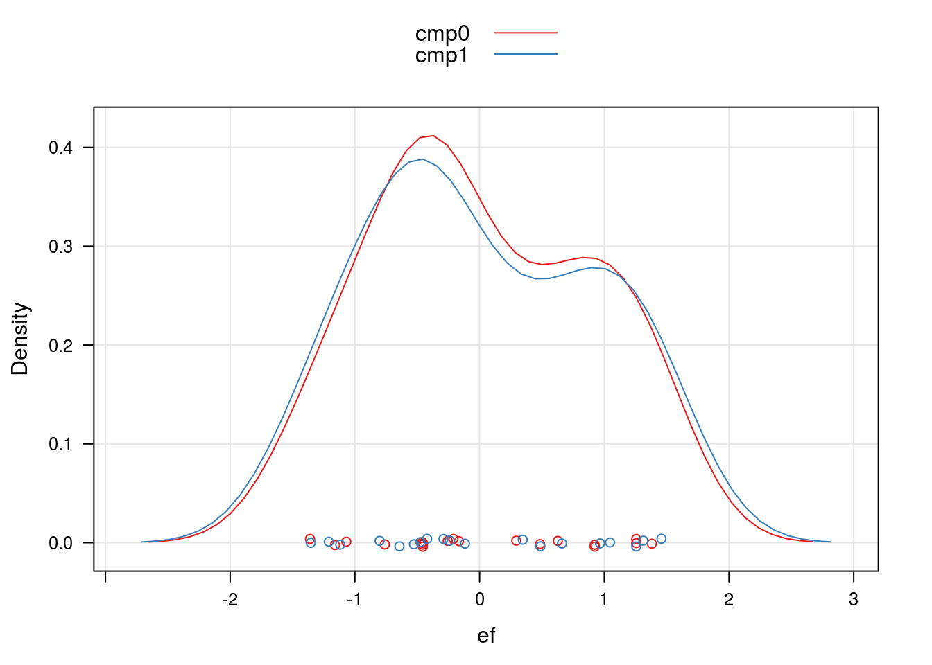

Abordagem Bayesiana com INLA

Modelo misto Poisson

##----------------------------------------------------------------------
## Com a poisson
library(INLA)

## Loading required package: sp

## Loading required package: splines

inla0 <- inla(nema ~ 1 + f(cult, model = "iid"),
              data = nematodes, family = "poisson")
inla1 <- inla(nema ~ log(off) + f(cult, model = "iid"),
              data = nematodes, family = "poisson")

## Estimativas dos parametros
## Para o modelo sem efeito fixo
tinla0 <- rbind(c(sqrt(1/summary(inla0)$hyperpar[1]), rep(NA, 6)),
                summary(inla0)$fixed)
colnames(tinla0) <- colnames(summary(inla0)$fixed)
rownames(tinla0)[1] <- "sigma"
tinla0

##             mean     sd     0.025quant 0.5quant 0.975quant mode   kld
## sigma       0.729325 NA     NA         NA       NA         NA     NA 
## (Intercept) 1.7634   0.1793 1.4051     1.7647   2.1139     1.7671 0

## Para o modelo com efeito de off
tinla1 <- rbind(c(sqrt(1/summary(inla1)$hyperpar[1]), rep(NA, 6)),
                summary(inla1)$fixed)
colnames(tinla1) <- colnames(summary(inla1)$fixed)
rownames(tinla1)[1] <- "sigma"
tinla1

##             mean      sd     0.025quant 0.5quant 0.975quant mode   kld
## sigma       0.7018797 NA     NA         NA       NA         NA     NA 
## (Intercept) 2.1629    0.2321 1.7015     2.1646   2.6147     2.1678 0  
## log(off)    0.1632    0.0643 0.0374     0.163    0.2898     0.1626 0

## Predição para os efeitos aleatórios
ranef.inla0 <- data.frame(ef = inla0$summary.random$cult$mean,
                          m = "inla0")
ranef.inla1 <- data.frame(ef = inla1$summary.random$cult$mean,
                          m = "inla1")
ranef.inla <- rbind(ranef.inla0, ranef.inla1)

densityplot(~ef, groups = m,
            data = ranef.inla,
            axis = axis.grid,
            auto.key = TRUE)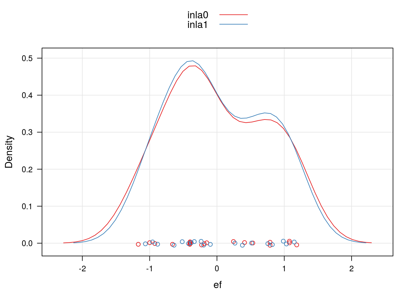

Modelo misto Gamma-Count

##----------------------------------------------------------------------
## Com a Gamma-Count
inlag0 <- inla(nema ~ 1 + f(cult, model = "iid"),
               data = nematodes, family = "gammacount")

## Warning in inla.model.properties.generic(inla.trim.family(model), (mm[names(mm) == : Model 'gammacount' in section 'likelihood' is marked as 'experimental'; changes may appear at any time.
##   Use this model with extra care!!! Further warnings are disabled.

inlag1 <- inla(nema ~ log(off) + f(cult, model = "iid"),
               data = nematodes, family = "gammacount")

## Estimativas dos parametros
## Para o modelo sem efeito fixo
tinlag0 <- rbind(c(sqrt(1/summary(inlag0)$hyperpar[2, 1]), rep(NA, 6)),
                 c(summary(inlag0)$hyperpar[2, 1], rep(NA, 6)),
                 summary(inlag0)$fixed)
colnames(tinlag0) <- colnames(summary(inlag0)$fixed)
rownames(tinlag0) <- c("sigma", "alpha", "(Intercept)")
tinlag0

##                  mean     sd 0.025quant 0.5quant 0.975quant   mode kld
## sigma       0.7262411     NA         NA       NA         NA     NA  NA
## alpha       1.8960000     NA         NA       NA         NA     NA  NA
## (Intercept) 1.7718000 0.1803     1.4084   1.7737     2.1239 1.7774   0

## Para o modelo com efeito de off
tinlag1 <- rbind(c(sqrt(1/summary(inlag1)$hyperpar[2, 1]), rep(NA, 6)),
                 c(summary(inlag1)$hyperpar[2, 1], rep(NA, 6)),
                 summary(inlag1)$fixed)
colnames(tinlag1) <- colnames(summary(inlag1)$fixed)
rownames(tinlag1) <- c("sigma", "alpha", "(Intercept)", "log(off)")
tinlag1

##                  mean     sd 0.025quant 0.5quant 0.975quant   mode kld
## sigma       0.6989248     NA         NA       NA         NA     NA  NA
## alpha       2.0471000     NA         NA       NA         NA     NA  NA
## (Intercept) 2.1668000 0.2251     1.7161   2.1691     2.6041 2.1735   0
## log(off)    0.1598000 0.0598     0.0433   0.1593     0.2785 0.1585   0

## Predição para os efeitos aleatórios
ranef.inlag0 <- data.frame(ef = inlag0$summary.random$cult$mean,
                          m = "inlag0")
ranef.inlag1 <- data.frame(ef = inlag1$summary.random$cult$mean,
                          m = "inlag1")
ranef.inlag <- rbind(ranef.inlag0, ranef.inlag1)

densityplot(~ef, groups = m,
            data = ranef.inlag,
            axis = axis.grid,
            auto.key = TRUE)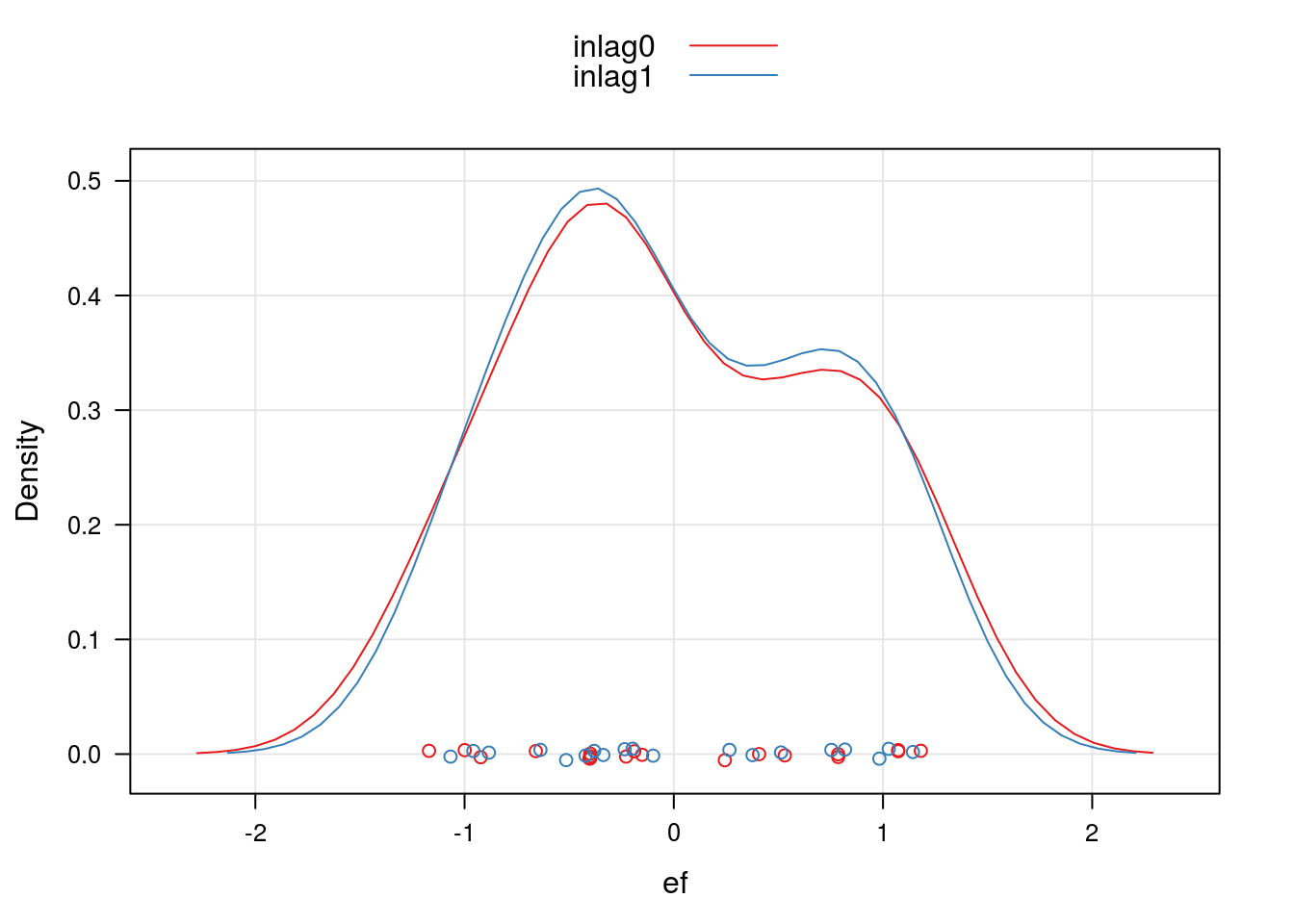

Abordagem Bayesiana por simulação

Funções para facilitar a análise das amostras da simulação.

##======================================================================
## Por amostragem MCMC
library(rjags)

## Linked to JAGS 4.2.0

## Loaded modules: basemod,bugs

select_pars <- function(sample, pars) {
    if (!is.mcmc.list(sample)) {
        sample <- as.mcmc.list(sample)
    }
    out <- lapply(sample, function(x) {
        sel <- gsub("\\[[0-9]+\\]", repl = "", colnames(x))
        x[, sel %in% pars]
    })
    return(as.mcmc(out))
}

Modelo misto Poisson

Abaixo define-se o modelo conforme sintaxe do JAGS

##-------------------------------------------
## Com a Poisson (Modelo sem efeito de covariavel)
poisRE0 <-
" model {
    ## Log-verossimilhanca
    for (i in 1:m) {
      u[i] ~ dnorm(0, tau.e)
    }
    for (j in 1:n) {
      log(mu[j]) <- b0 + u[ind[j]]
      y[j] ~ dpois(mu[j])
    }
    ## Prioris
    b0 ~ dnorm(0, 0.0001)
    tau.e ~ dgamma(0.001, 0.001)
    sigma <- sqrt(1/tau.e)
}
"

##-------------------------------------------
## Modelo sem efeito de covariavel
data0 <- with(
    nematodes,
    list("y" = nema,
         "n" = length(nema),
         "m" = length(unique(cult)),
         "ind" = as.numeric(cult))
)

jagsmodel0 <- jags.model(
    textConnection(poisRE0),
    data = data0,
    n.chains = 3,
    n.adapt = 1000
)

amostra0 <- coda.samples(
    jagsmodel0, c("b0", "sigma", "u", "mu"),
    n.iter = 10000, thin = 10,
    n.chains = 3,
    n.adapt = 1000)

Avaliação das cadeias

## Seleciona apenas os parâmetros amostrados do modelo
ampars0 <- select_pars(amostra0, pars = c("b0", "sigma"))

## Gráficos de diagnóstico
xyplot(ampars0, axis = axis.grid, aspect = "fill")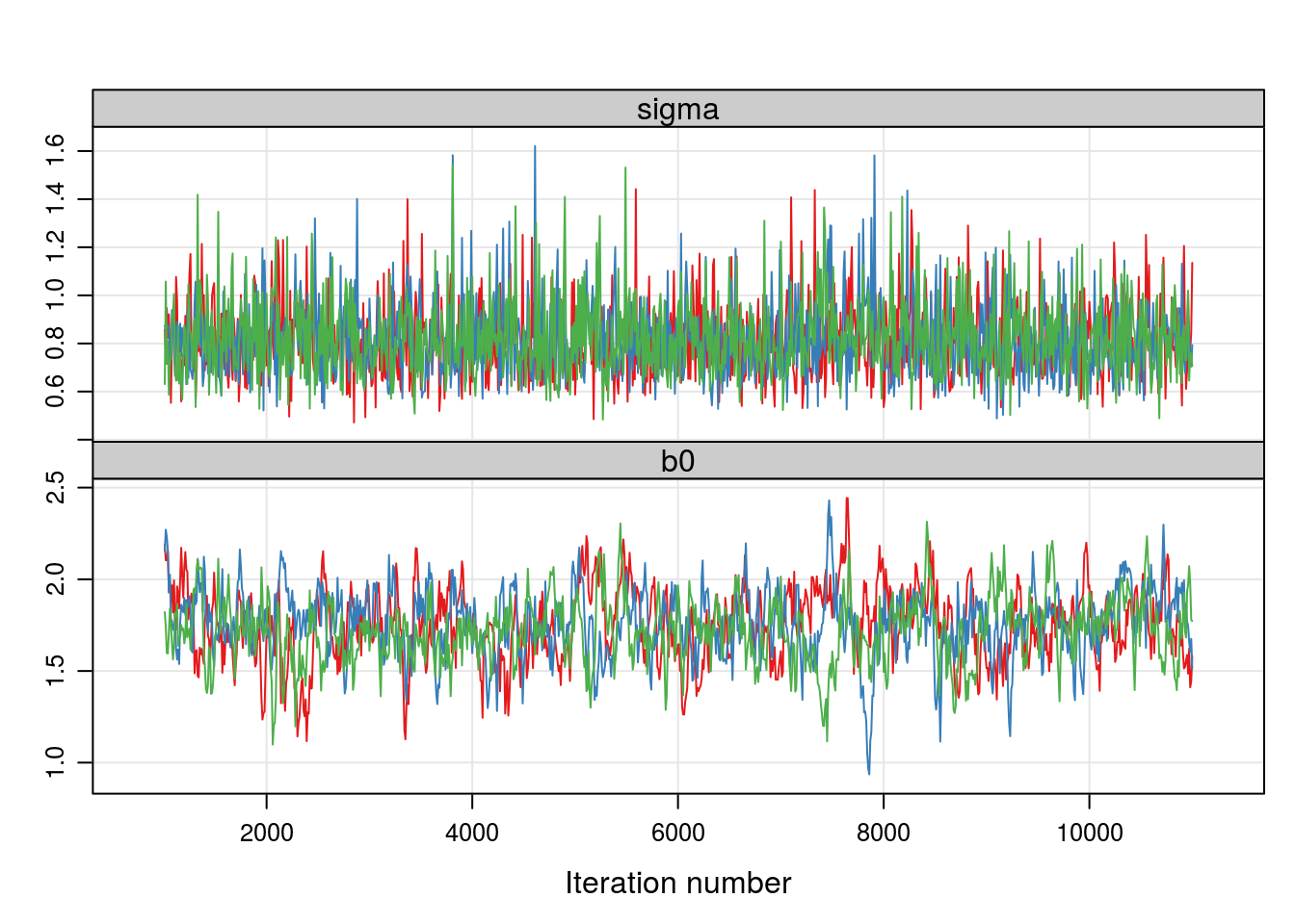

densityplot(ampars0, axis = axis.grid, aspect = "fill")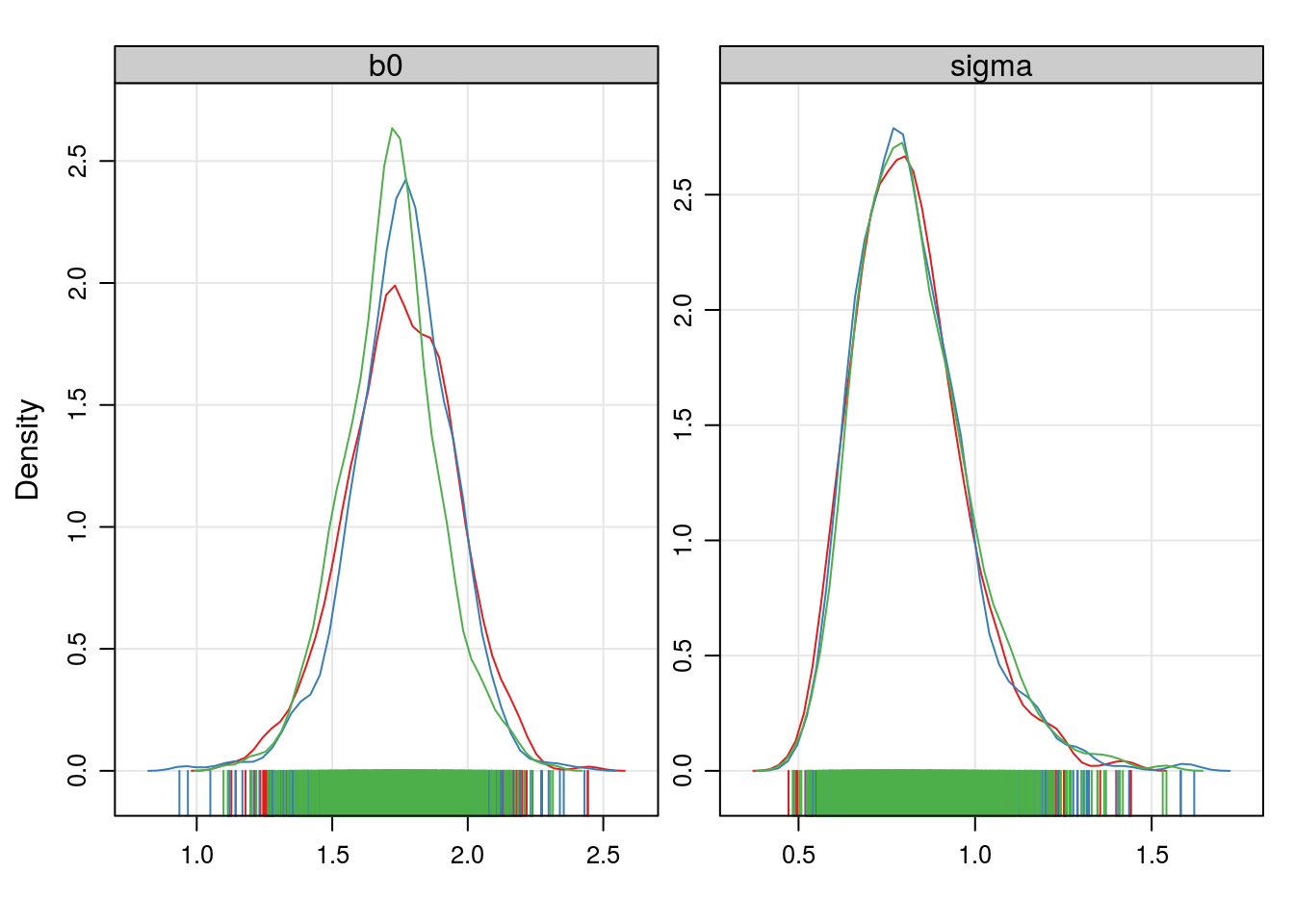

acfplot(ampars0, type = "h", axis = axis.grid, aspect = "fill")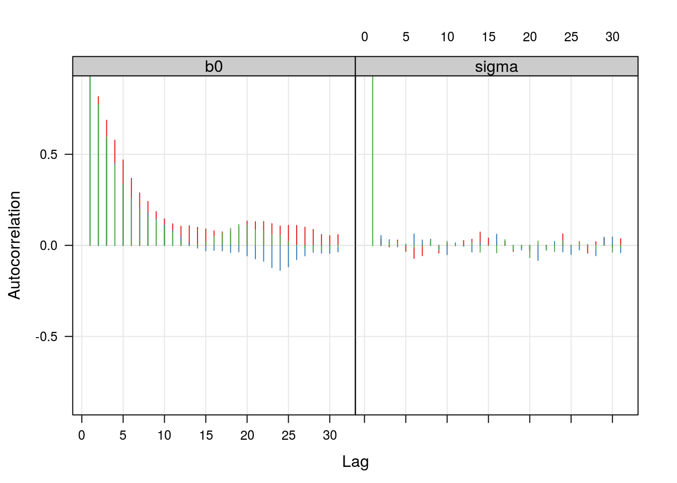

Resumos da posteriori

##-------------------------------------------
## Resumos da posteriori (para os parametros b0 e sigma)

ampars0 <- as.mcmc(do.call(rbind, ampars0))

(resumo0 <- summary(ampars0)$statistics)

##            Mean        SD    Naive SE Time-series SE
## b0    1.7429911 0.1888004 0.003447007    0.010060598
## sigma 0.8183629 0.1556370 0.002841529    0.002932447

HPDinterval(ampars0)

##           lower    upper
## b0    1.3621824 2.112360
## sigma 0.5282123 1.113475
## attr(,"Probability")
## [1] 0.95

Predição dos efeitos aleatórios

amranef0 <- select_pars(amostra0, pars = "u")
amranef0 <- as.mcmc(do.call(rbind, amranef0))
ranef.jags0 <- data.frame(
    ef = summary(amranef0)$statistics[, 1],
    m = "jags0")

qqmath(~ef, data = ranef.inlag0,
       axis = axis.grid,
       panel = function(...) {
           panel.qqmath(...)
           panel.qqmathline(..., lty = 2, col = "gray50")
       })

Define o modelo com o efeito de covariável

##-------------------------------------------
## Com a Poisson (modelo com covariável)
poisRE1 <-
" model {
    ## Log-verossimilhanca
    for (i in 1:m) {
      u[i] ~ dnorm(0, tau.e)
    }
    for (j in 1:n) {
      log(mu[j]) <- b0 + b1 * cov[j] + u[ind[j]]
      y[j] ~ dpois(mu[j])
    }
    ## Prioris
    b0 ~ dnorm(0, 0.0001)
    b1 ~ dnorm(0, 0.0001)
    tau.e ~ dgamma(0.001, 0.001)
    sigma <- sqrt(1/tau.e)
}
"

##-------------------------------------------
## Modelo com efeito de covariavel
data1 <- with(
    nematodes,
    list("y" = nema,
         "cov" = log(off),
         "n" = length(nema),
         "m" = length(unique(cult)),
         "ind" = as.numeric(cult))
)

jagsmodel1 <- jags.model(
    textConnection(poisRE1),
    data = data1,
    n.chains = 3,
    n.adapt = 1000
)

amostra1 <- coda.samples(
    jagsmodel1, c("b0", "b1", "sigma", "u", "mu"),
    n.iter = 15000, thin = 15,
    n.chains = 3,
    n.adapt = 1000)

Avaliação da cadeia

##-------------------------------------------
## Avaliação das cadeias
ampars1 <- select_pars(amostra1, pars = c("b0", "b1", "sigma"))

xyplot(ampars1, axis = axis.grid, aspect = "fill")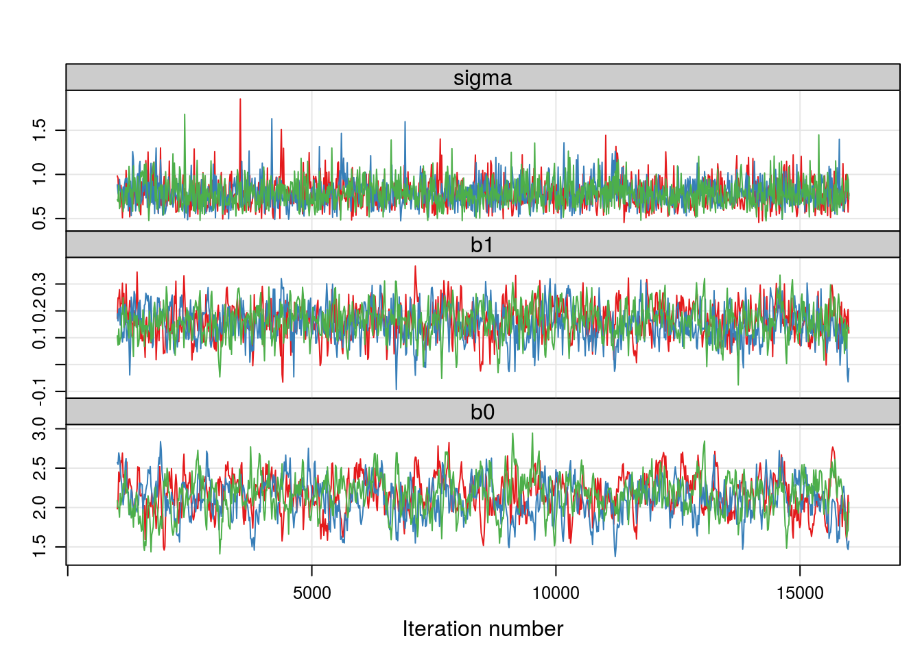

densityplot(ampars1, axis = axis.grid, aspect = "fill")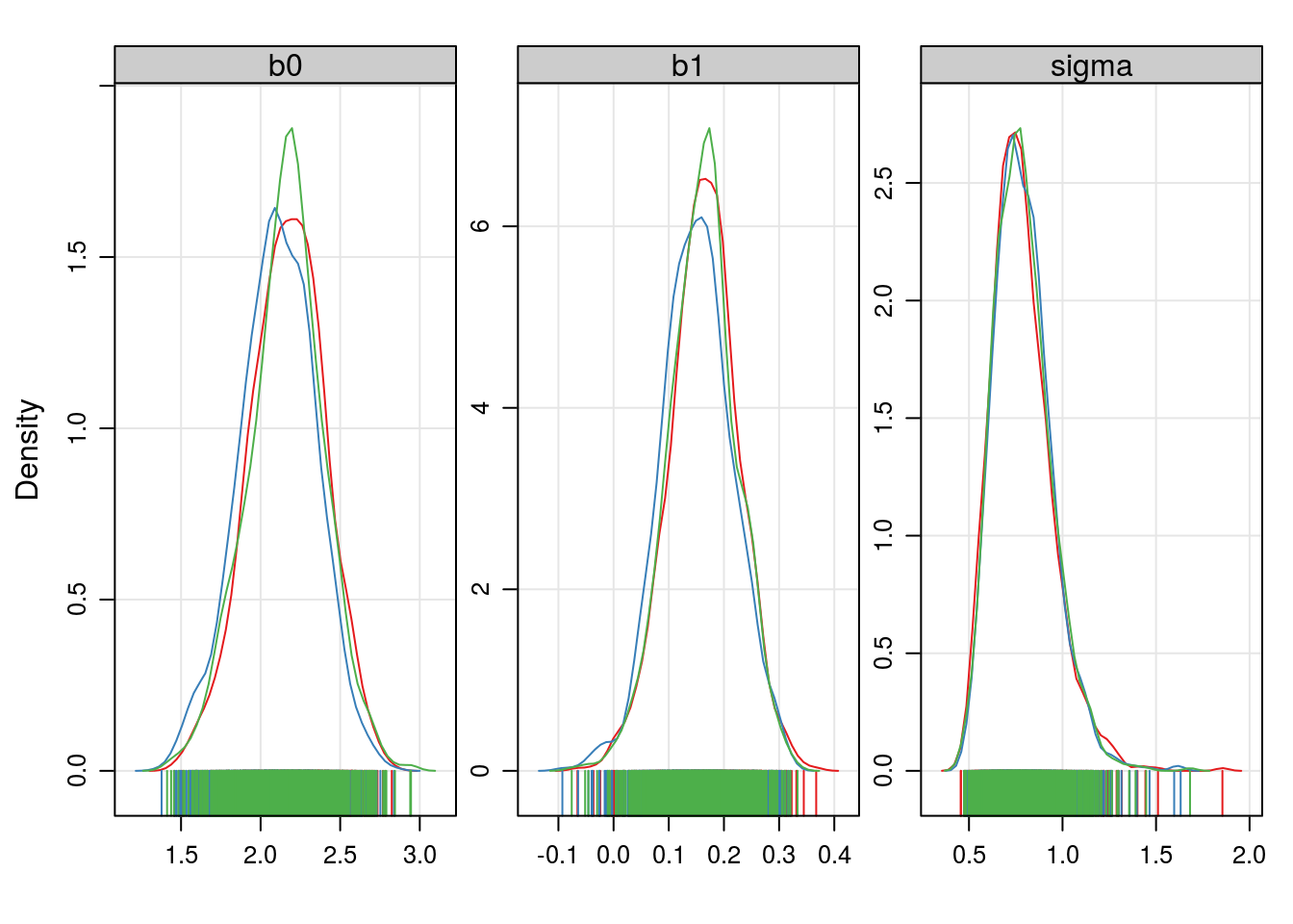

acfplot(ampars1, type = "h", axis = axis.grid, aspect = "fill")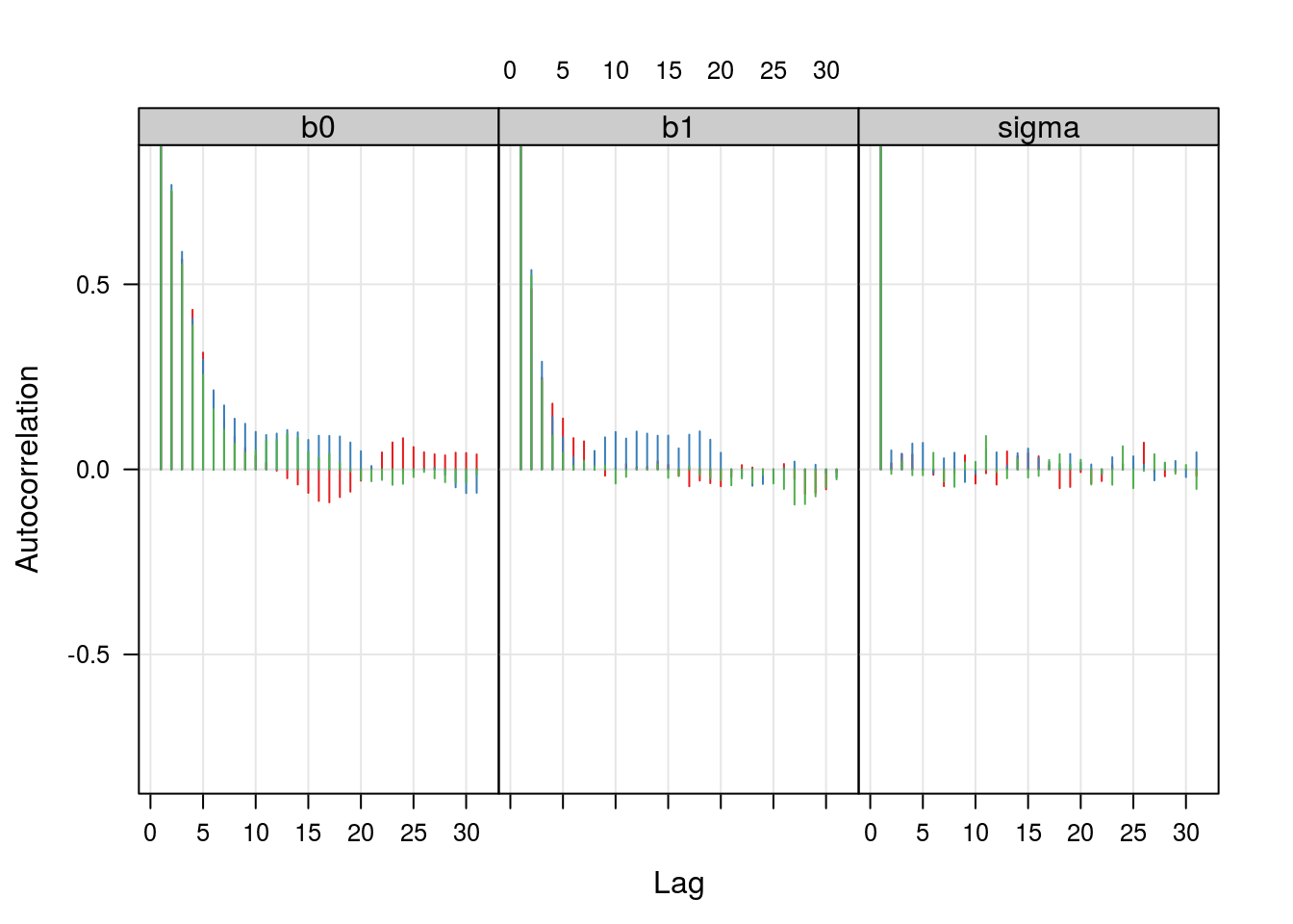

Resumos da posteriori

## Resumos da posteriori (para os parametros b0, b1 e sigma)

ampars1 <- as.mcmc(do.call(rbind, ampars1))

(resumo1 <- summary(ampars1)$statistics)

##            Mean         SD    Naive SE Time-series SE
## b0    2.1445086 0.23854378 0.004355194     0.01121614
## b1    0.1586287 0.06292222 0.001148797     0.00204875
## sigma 0.7884180 0.15568930 0.002842485     0.00309550

HPDinterval(ampars1)

##            lower     upper
## b0    1.65203156 2.6032257
## b1    0.03478347 0.2826243
## sigma 0.51363772 1.0971334
## attr(,"Probability")
## [1] 0.95

Predição dos efeitos aleatórios

##-------------------------------------------
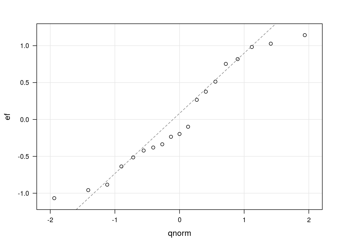
## Predição dos efeitos aleatórios
amranef1 <- select_pars(amostra1, pars = "u")
amranef1 <- as.mcmc(do.call(rbind, amranef1))
ranef.jags1 <- data.frame(
    ef = summary(amranef1)$statistics[, 1],
    m = "jags1")

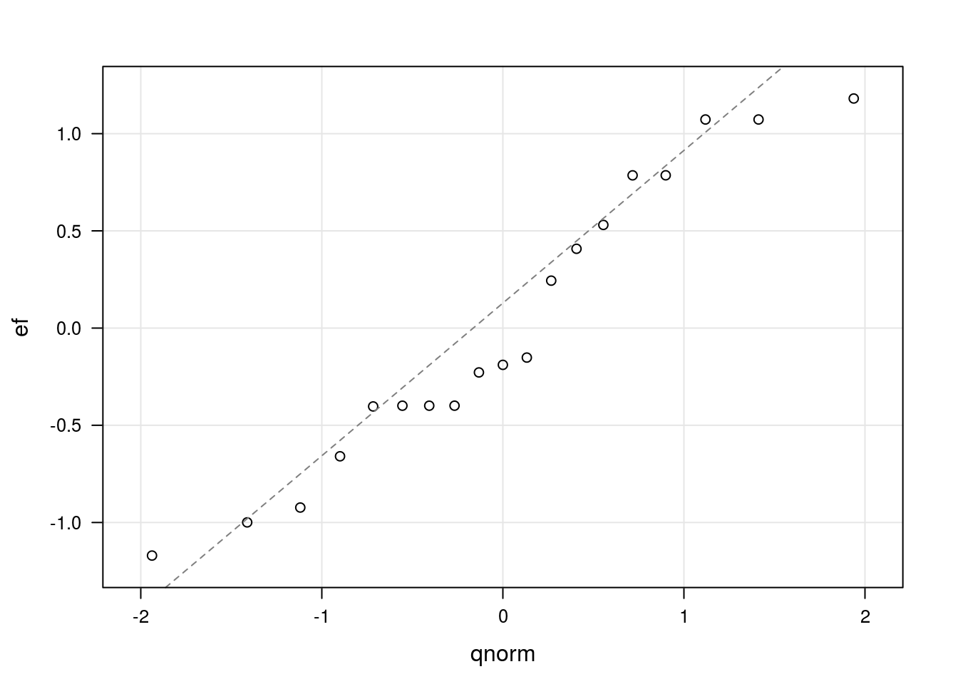
qqmath(~ef, data = ranef.inlag1,
       axis = axis.grid,
       panel = function(...) {
           panel.qqmath(...)
           panel.qqmathline(..., lty = 2, col = "gray50")
       })

Comparando os efeitos aleatórios

##-------------------------------------------
## Empilhando os efeitos aleatórios
ranef.jags <- rbind(ranef.jags0, ranef.jags1)

densityplot(~ef, groups = m,
            data = ranef.jags,
            axis = axis.grid,
            auto.key = TRUE)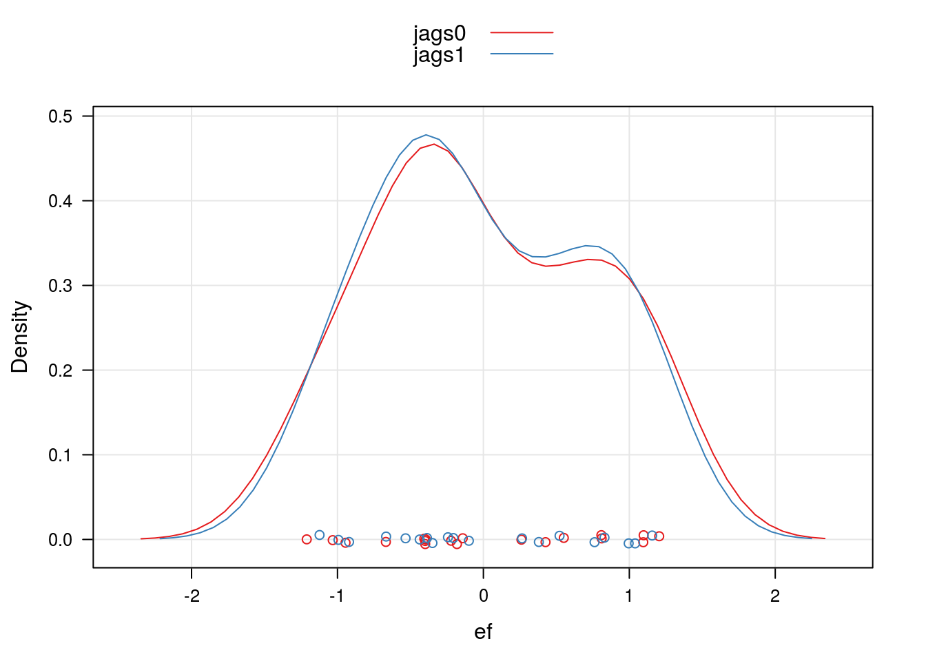

Comparação

tmle0

##             Estimate Std. Error  z value
## sigma       0.759144         NA       NA
## (Intercept) 1.760503  0.1808152 9.736474

tcmp0

##              Estimate Std. Error   z value
## sigma       0.8749274         NA        NA
## phi         0.1528742  0.1792980 0.8526264
## (Intercept) 2.0683427  0.4408113 4.6921272

tinla0

##             mean     sd     0.025quant 0.5quant 0.975quant mode   kld
## sigma       0.729325 NA     NA         NA       NA         NA     NA 
## (Intercept) 1.7634   0.1793 1.4051     1.7647   2.1139     1.7671 0

tinlag0

##                  mean     sd 0.025quant 0.5quant 0.975quant   mode kld
## sigma       0.7262411     NA         NA       NA         NA     NA  NA
## alpha       1.8960000     NA         NA       NA         NA     NA  NA
## (Intercept) 1.7718000 0.1803     1.4084   1.7737     2.1239 1.7774   0

resumo0

##            Mean        SD    Naive SE Time-series SE
## b0    1.7429911 0.1888004 0.003447007    0.010060598
## sigma 0.8183629 0.1556370 0.002841529    0.002932447

tmle1

##              Estimate Std. Error  z value
## sigma       0.7310786         NA       NA
## (Intercept) 2.1562623 0.23278215 9.263005
## log(off)    0.1620083 0.06397819 2.532242

tcmp1

##              Estimate Std. Error  z value
## sigma       0.9161159         NA       NA
## phi         0.2409883 0.17683814 1.362762
## (Intercept) 2.7523952 0.56492336 4.872157
## log(off)    0.1982931 0.07807116 2.539902

tinla1

##             mean      sd     0.025quant 0.5quant 0.975quant mode   kld
## sigma       0.7018797 NA     NA         NA       NA         NA     NA 
## (Intercept) 2.1629    0.2321 1.7015     2.1646   2.6147     2.1678 0  
## log(off)    0.1632    0.0643 0.0374     0.163    0.2898     0.1626 0

tinlag1

##                  mean     sd 0.025quant 0.5quant 0.975quant   mode kld
## sigma       0.6989248     NA         NA       NA         NA     NA  NA
## alpha       2.0471000     NA         NA       NA         NA     NA  NA
## (Intercept) 2.1668000 0.2251     1.7161   2.1691     2.6041 2.1735   0
## log(off)    0.1598000 0.0598     0.0433   0.1593     0.2785 0.1585   0

resumo1

##            Mean         SD    Naive SE Time-series SE
## b0    2.1445086 0.23854378 0.004355194     0.01121614
## b1    0.1586287 0.06292222 0.001148797     0.00204875
## sigma 0.7884180 0.15568930 0.002842485     0.00309550

Inferência Bayesiana - Análise de experimento com via inferência clássica e Bayesiana

Eduardo E. R. Junior - DEST/UFPR

22 de junho de 2016

Definição do problema

Modelos em competição

Abordagem de Máxima Verossimilhança

Modelo misto Poisson

Modelo misto COM-Poisson

Abordagem Bayesiana com INLA

Modelo misto Poisson

Modelo misto Gamma-Count

Abordagem Bayesiana por simulação

Modelo misto Poisson

Comparação